Dynamic Connectivity and Percolation

By Kumar Utsav · April 07, 2022 · 12 minutes

Given a set of N objects that support the following two commands:

Union: Connect two objects.
Find/Connected: Is there a path connecting the two obejcts?

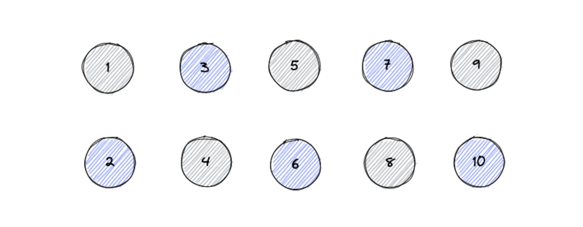
For example, consider this set of 10 objects

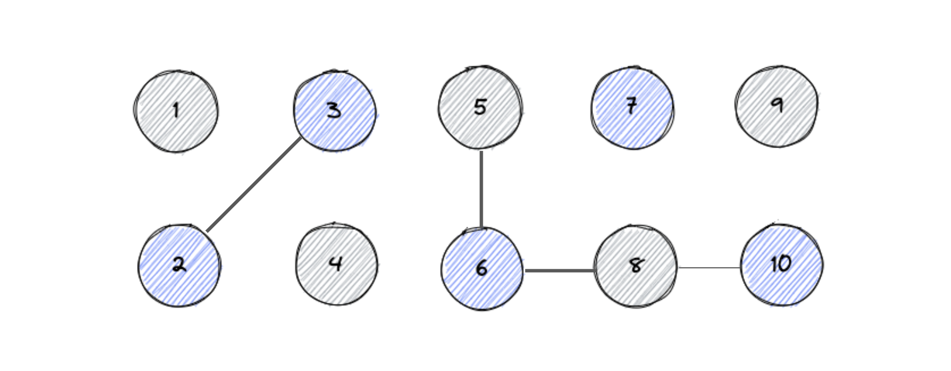
After few union commands union(2, 3), union(6, 5), union(8, 6), union(10, 8) the state of the system changes to

We can query the above system to find if two objects are connected or not like find(0, 1) == False, find(1, 2) == True, find(4, 9) == True, find(8, 1) == False

To be formal, we can say that “connected to” has the following properties:

Reflexive: a is connected to a.
Symmetric: if a is connected to b, then b is conntected to a.
Transitive: if a is connected to b and b is conntected to c, then a is connected to c.

Another common terminology in dynamic connectivity problems is Connected components. It refers to the maximal set of objects that are mutually connected. In the above example, the conntected components are {0}, {1, 2}, {3}, {4, 5, 7, 9}, {6}, {8}. The union-find algorithms we are going to implement below can help us model objects of many different kinds. Some of the practical examples include:

Pixels in an image.
Computers in a network.
Friends in a network.
Grid system for path finding problems.

When we are programming the union-find operations, it’s convenient to represent the set of objects and their connectivity using a list from 0 to N-1. The overall goal is to design a data structure and algorithm for union-find that is effecient when:

Number of ojects N can be huge.
Number of operations M can be huge.
Find and Union queries can be intermixed.

Quick-Find

We will used id[] to store all the obecjts. The index will refer to the objects and the value will indicate the connectivity between two indices.

For example id[] = [0, 1, 1, 3, 5, 5, 6, 5, 8, 5]. Here, objects {1, 2} are connected and {4, 5, 7, 9} are connected.

Find: Check if indices a and b have the same id.
Union: To merge indices a and b, change all entries whose id equals id[a] to id[b].

 1
 2
 3
 4
 5
 6
 7
 8
 9
10
11
12
13
14


from collections import defaultdict, Counter
import random
import time

import matplotlib.pyplot as plt
import numpy as np


def plot(sequences):
    plt.figure(figsize=(12, 6))
    for k, seq, label in sequences:
        plt.plot(k, seq, label=label)
    plt.legend()
    return plt

 1
 2
 3
 4
 5
 6
 7
 8
 9
10
11
12
13
14
15
16
17
18
19
20
21
22
23
24
25
26
27
28
29
30
31
32
33
34


class QuickFind:

    def __init__(self, n:int=10):
        self.id = list(range(n))

    def __getitem__(self, ix:int) -> int:
        return self.id[ix]

    def __len__(self) -> int:
        return len(self.id)

    def find(self, a:int, b:int) -> bool:
        return self.id[a] == self.id[b]

    def union(self, a:int, b:int) -> None:
        root_of_a = self.id[a]
        root_of_b = self.id[b]
        for i, _ in enumerate(self.id):
            if self.id[i] == root_of_a:
                self.id[i] = root_of_b

    def simulate(self) -> None:
        n = len(self.id)
        for _ in range(n):
            a = random.randint(0, n-1)
            b = random.randint(0, n-1)
            if random.random() > 0.5:
                st = time.time()
                self.union(a, b)
                timings["union"][n].append(time.time() - st)
            else:
                st = time.time()
                self.find(a, b)
                timings["find"][n].append(time.time() - st)

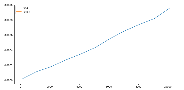
It’s easy to observe the worst case time complexity of QuickFind:

Initialize: O(N)
Union: O(N)
Find: O(1)

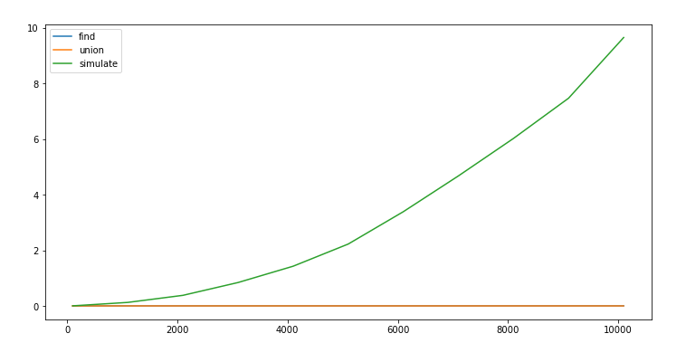
Even though the operations don’t look too bad on their own, for a sequence of N union commands on N objects(a very common operation for such problems), this becomes O(N^2).

1
2
3
4
5
6
7
8
9


timings = {"find": defaultdict(list), "union": defaultdict(list), "simulate": []}

print("simulating ", end="")
for i in range(100, 11000, 1000):
    print(i, end=" ")
    qf = QuickFind(i)
    st = time.time()
    qf.simulate()
    timings["simulate"].append(time.time() - st)

simulating 100 1100 2100 3100 4100 5100 6100 7100 8100 9100 10100

1
2
3


plot([(timings["find"].keys(), [np.mean(v) for t, v in timings["find"].items()], "find"),
      (timings["union"].keys(), [np.mean(v) for t, v in timings["union"].items()], "union")
]);

png

1
2
3
4


plot([(timings["find"].keys(), [np.mean(v) for t, v in timings["find"].items()], "find"),
      (timings["union"].keys(), [np.mean(v) for t, v in timings["union"].items()], "union"),
      (timings["union"].keys(), timings["simulate"], "simulate")
]);

png

An improvement over QuickFind is the QuickUnion algorithm.

Quick-Union

Here also we use an array to store the objects, though the interpretation of the values in the array changes, nowid[i] is the parent of i. We are essentially using the array to create a tree like structure. To find the root of any object i, we recursively traverse it’s parent till the index is same as the value, i.e. Root of i is id[id[id[…id[i]…]]].

 1
 2
 3
 4
 5
 6
 7
 8
 9
10
11
12
13
14
15
16
17
18
19
20
21
22
23
24
25
26
27
28
29
30
31
32
33
34
35
36
37
38
39
40
41
42
43
44
45
46
47
48


class QuickUnion:

    def __init__(self, n:int=10):
        self.id = list(range(n))

    def __getitem__(self, ix:int) -> int:
        return self.id[ix]

    def __len__(self) -> int:
        return len(self.id)

    def root(self, ix:int) -> int:
        while ix != self.id[ix]:
            ix = self.id[ix]
        return ix

    def find(self, a:int, b:int) -> bool:
        return self.root(a) == self.root(b)

    def union(self, a:int, b:int) -> None:
        root_of_a = self.root(a)
        root_of_b = self.root(b)
        self.id[root_of_a] = root_of_b

    def simulate(self) -> None:
        n = len(self.id)
        for _ in range(n):
            a = random.randint(0, n-1)
            b = random.randint(0, n-1)
            if random.random() > 0.5:
                st = time.time()
                self.union(a, b)
                timings["union"][n].append(time.time() - st)
            else:
                st = time.time()
                self.find(a, b)
                timings["find"][n].append(time.time() - st)

    def simulate_worst_case(self) -> None:
        n = len(self.id)
        for i in range(n-1):
            st = time.time()
            self.union(i, i+1)
            timings["union"][n].append(time.time() - st)
        for i in range(n):
            st = time.time()
            self.find(i, i)
            timings["find"][n].append(time.time() - st)

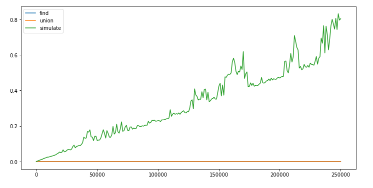
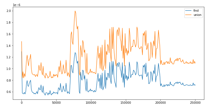
Here we can observe that the Union and Find operations have a time complexity of O(logN) on average, given that the tree remains balanced. The problem occurs when the tree gets too tall. In the worst case, we can end up with one very tall skinny tree where the time complexity of Find operation becomes O(N). In this case, we again end up with O(N^2) for N finds on N objects.

So in the worst case:

Initialize: O(N)
Union: O(N)
Find: O(N)

Average Case

 1
 2
 3
 4
 5
 6
 7
 8
 9
10


timings = {"find": defaultdict(list), "union": defaultdict(list), "simulate": []}

print("simulating ", end="")
for i in range(100, 251000, 1000):
    if int(str(i)[:2]) % 11 == 0:
        print(i, end=" ")
    qu = QuickUnion(i)
    st = time.time()
    qu.simulate()
    timings["simulate"].append(time.time() - st)

simulating 1100 11100 22100 33100 44100 55100 66100 77100 88100 99100 110100 111100 112100
113100 114100 115100 116100 117100 118100 119100 220100 221100 222100 223100 224100 225100
226100 227100 228100 229100

1
2
3


plot([(timings["find"].keys(), [np.mean(v) for t, v in timings["find"].items()], "find"),
      (timings["union"].keys(), [np.mean(v) for t, v in timings["union"].items()], "union")
]);

png

1
2
3
4


plot([(timings["find"].keys(), [np.mean(v) for t, v in timings["find"].items()], "find"),
      (timings["union"].keys(), [np.mean(v) for t, v in timings["union"].items()], "union"),
      (timings["union"].keys(), timings["simulate"], "simulate")
]);

png

Worst case

1
2
3
4
5
6
7
8
9


timings = {"find": defaultdict(list), "union": defaultdict(list), "simulate": []}

print("simulating ", end="")
for i in range(100, 11000, 1000):
    print(i, end=" ")
    qu = QuickUnion(i)
    st = time.time()
    qu.simulate_worst_case()
    timings["simulate"].append(time.time() - st)

simulating 100 1100 2100 3100 4100 5100 6100 7100 8100 9100 10100

1
2
3


plot([(timings["find"].keys(), [np.mean(v) for t, v in timings["find"].items()], "find"),
      (timings["union"].keys(), [np.mean(v) for t, v in timings["union"].items()], "union")
]);

png

1
2
3
4


plot([(timings["find"].keys(), [np.mean(v) for t, v in timings["find"].items()], "find"),
      (timings["union"].keys(), [np.mean(v) for t, v in timings["union"].items()], "union"),
      (timings["union"].keys(), timings["simulate"], "simulate")
]);

png

Quick-Union-Weighted

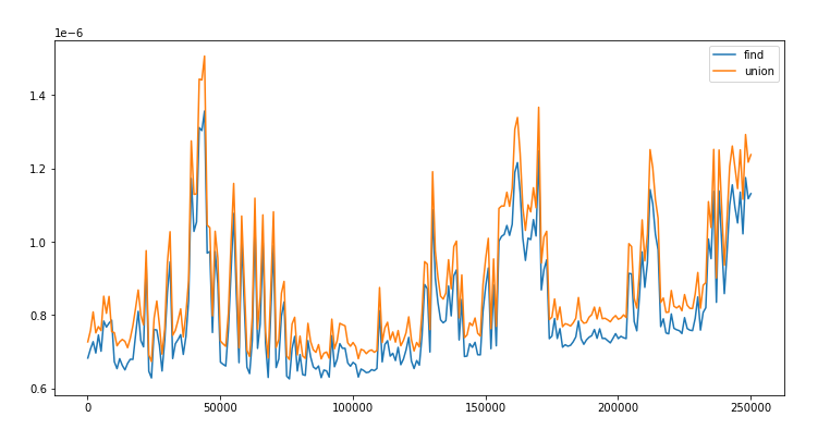
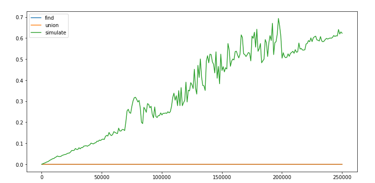
The QuickUnion can easily be improved by trying to keep the trees balanced as the number of operations grow.

This can be done by keeping track of the size of the trees and using it for each union(a, b) operation. Now, instead of just changing the root of a to root of b, we compare the size of tree at a and the tree at b to decide whose root changes.

In the worst case now:

Initialize: O(N)
Union: O(logN)
Find: O(logN)

 1
 2
 3
 4
 5
 6
 7
 8
 9
10
11
12
13
14
15
16
17
18
19
20
21
22
23
24
25
26
27
28
29
30
31
32
33
34
35
36
37
38
39
40
41
42
43
44
45
46
47
48
49
50
51
52
53
54
55
56
57
58
59
60


class QuickUnionWeighted:

    def __init__(self, n:int=10):
        self.id = list(range(n))
        self._sizes = [1] * n

    def __getitem__(self, ix:int) -> int:
        return self.id[ix]

    def __len__(self) -> int:
        return len(self.id)

    def root(self, ix:int) -> int:
        while ix != self.id[ix]:
            ix = self.id[ix]
        return ix

    def find(self, a:int, b:int) -> bool:
        return self.root(a) == self.root(b)

    def union(self, a:int, b:int) -> None:
        root_of_a = self.root(a)
        root_of_b = self.root(b)
        if root_of_a == root_of_b:
            return
        if self._sizes[root_of_a] > self._sizes[root_of_b]:
            self._sizes[root_of_a] += self._sizes[root_of_b]
            self.id[root_of_b] = root_of_a
        else:
            self._sizes[root_of_b] += self._sizes[root_of_a]
            self.id[root_of_a] = root_of_b

    def simulate(self) -> None:
        n = len(self.id)
        for _ in range(n):
            a = random.randint(0, n-1)
            b = random.randint(0, n-1)
            if random.random() > 0.5:
                st = time.time()
                self.union(a, b)
                timings["union"][n].append(time.time() - st)
            else:
                st = time.time()
                self.find(a, b)
                timings["find"][n].append(time.time() - st)

    def simulate_worst_case(self) -> None:
        n = len(self.id)
        for _ in range(n):
            a = random.randint(0, n-1)
            b = random.randint(0, n-1)
            st = time.time()
            self.union(a, b)
            timings["union"][n].append(time.time() - st)
        for _ in range(n):
            a = random.randint(0, n-1)
            b = random.randint(0, n-1)
            st = time.time()
            self.find(a, b)
            timings["find"][n].append(time.time() - st)

With balanced trees, for N Find operations over N objects, our worst time complexity should be O(NlogN).

 1
 2
 3
 4
 5
 6
 7
 8
 9
10


timings = {"find": defaultdict(list), "union": defaultdict(list), "simulate": []}

print("simulating ", end="")
for i in range(100, 251000, 1000):
    if int(str(i)[:2]) % 11 == 0:
        print(i, end=" ")
    quw = QuickUnionWeighted(i)
    st = time.time()
    quw.simulate()
    timings["simulate"].append(time.time() - st)

simulating 1100 11100 22100 33100 44100 55100 66100 77100 88100 99100 110100 111100 112100
113100 114100 115100 116100 117100 118100 119100 220100 221100 222100 223100 224100 225100
226100 227100 228100 229100

1
2
3


plot([(timings["find"].keys(), [np.mean(v) for t, v in timings["find"].items()], "find"),
      (timings["union"].keys(), [np.mean(v) for t, v in timings["union"].items()], "union")
]);

png

1
2
3
4


plot([(timings["find"].keys(), [np.mean(v) for t, v in timings["find"].items()], "find"),
      (timings["union"].keys(), [np.mean(v) for t, v in timings["union"].items()], "union"),
      (timings["union"].keys(), timings["simulate"], "simulate")
]);

png

 1
 2
 3
 4
 5
 6
 7
 8
 9
10


timings = {"find": defaultdict(list), "union": defaultdict(list), "simulate": []}

print("simulating ", end="")
for i in range(100, 251000, 1000):
    if int(str(i)[:2]) % 11 == 0:
        print(i, end=" ")
    quw = QuickUnionWeighted(i)
    st = time.time()
    quw.simulate_worst_case()
    timings["simulate"].append(time.time() - st)

simulating 1100 11100 22100 33100 44100 55100 66100 77100 88100 99100 110100 111100 112100
113100 114100 115100 116100 117100 118100 119100 220100 221100 222100 223100 224100 225100
226100 227100 228100 229100

1
2
3


plot([(timings["find"].keys(), [np.mean(v) for t, v in timings["find"].items()], "find"),
      (timings["union"].keys(), [np.mean(v) for t, v in timings["union"].items()], "union")
]);

png

1
2
3
4


plot([(timings["find"].keys(), [np.mean(v) for t, v in timings["find"].items()], "find"),
      (timings["union"].keys(), [np.mean(v) for t, v in timings["union"].items()], "union"),
      (timings["union"].keys(), timings["simulate"], "simulate")
]);

png

Percolation

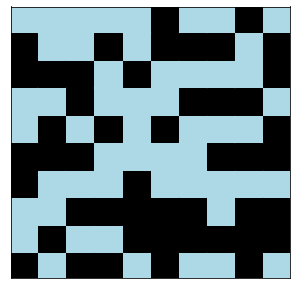
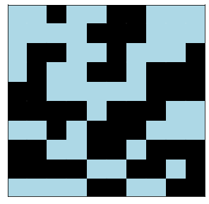
Percolation is a model for many physical systems. The system can be represented in the following way:

N-by-N grid of sites.
Each site is open with probability p (or blocked with probability 1-p).
System percolates if the top and bottom are connected by open sites.

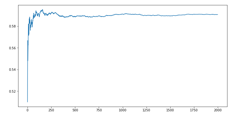
One example can be water flowing through a block of bricks with open sites indicating porus material. The likelihood of percolation depends on the site vacancy probability p. We will use the QuickUnionWeighted algorithm to find the threshold for p where the liklehood of percolation changes suddenly from 0 to 1.

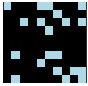
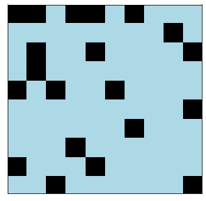
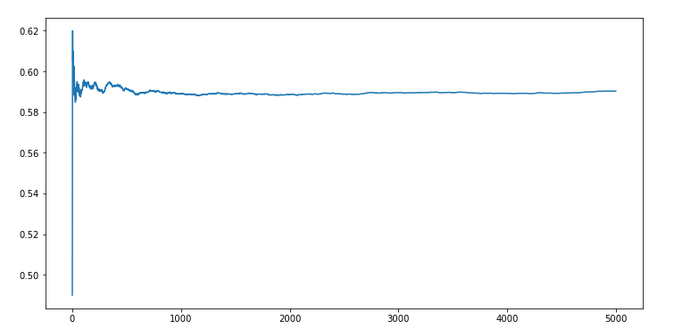
We will run monte carlo simulation on a system:

Which starts with all sites blocked.
In each step, we randomly open a site and check if the system percolates.
We keep repeating the last step till the system percolates.
We estimate p as (# open sites) / (N * N).
Repeat the above steps M(1000x) times.

If there is such a threshold for p where “the liklehood of percolation changes suddenly from 0 to 1”, then a running mean of all the p over multiple simulations should give us that number according to the law of large numbers.

 1
 2
 3
 4
 5
 6
 7
 8
 9
10
11
12
13
14
15
16
17
18
19
20
21
22
23
24
25
26
27
28
29
30
31
32
33
34
35
36
37
38
39
40
41
42
43
44
45
46
47
48
49
50
51
52
53
54
55
56
57
58
59
60
61
62
63
64
65
66
67
68
69
70
71
72
73
74
75
76
77
78
79
80
81
82
83
84
85
86
87
88
89
90
91
92
93
94


class PercolationModel:

    def __init__(self, n:int=10):
        self.id = list(range(n))
        self._sizes = [1] * n
        self._open = [0] * n
        self._ixs = list(range(n))
        self.n = int(np.sqrt(n))
        self.nxn = n

    def reset(self) -> None:
        self.id = list(range(self.nxn))
        self._sizes = [1] * self.nxn
        self._open = [0] * self.nxn
        self._ixs = list(range(self.nxn))

    def __getitem__(self, ix:int) -> int:
        return self.id[ix]

    def __len__(self) -> int:
        return len(self.id)

    def root(self, ix:int) -> int:
        while ix != self.id[ix]:
            ix = self.id[ix]
        return ix

    def find(self, a:int, b:int) -> bool:
        return self.root(a) == self.root(b)

    def is_valid_ix(self, r:int, c:int) -> bool:
        return (r > -1 and r < self.n) and (c > -1 and c < self.n)

    def union(self, a:int, b:int) -> None:
        root_of_a = self.root(a)
        root_of_b = self.root(b)
        if self._sizes[root_of_a] > self._sizes[root_of_b]:
            self._sizes[root_of_a] += self._sizes[root_of_b]
            self.id[root_of_b] = root_of_a
        else:
            self._sizes[root_of_b] += self._sizes[root_of_a]
            self.id[root_of_a] = root_of_b

    def open_site(self) -> None:
        ix = random.sample(self._ixs, 1)[0]
        self._ixs.remove(ix)
        self._open[ix] = 1
        r, c = ix // self.n, ix % self.n
        if self.is_valid_ix(r-1, c) and self._open[ix-self.n]: # up
            self.union(ix, ix-self.n)
        if self.is_valid_ix(r, c-1) and self._open[ix-1]: # left
            self.union(ix, ix-1)
        if self.is_valid_ix(r, c+1) and self._open[ix+1]: # right
            self.union(ix, ix+1)
        if self.is_valid_ix(r+1, c) and self._open[ix+self.n]: # down
            self.union(ix, ix+self.n)

    def percolates(self) -> bool:
        last_r = self.n * (self.n-1)
        for c1 in range(self.n):
            for c2 in range(self.n):
                if self.find(c1, last_r+c2):
                    return True
        return False

    def simulate(self, n_sims:int=1000, till_p=None) -> (float, list):
        p = [];
        for i in range(n_sims):
            self.reset()
            n_open_sites = 0
            if till_p:
                while (n_open_sites / self.nxn) < till_p:
                    self.open_site()
                    n_open_sites += 1
                p.append(n_open_sites / self.nxn)
            else:
                while not self.percolates():
                    self.open_site()
                    n_open_sites += 1
                p.append(n_open_sites / self.nxn)
        return np.mean(p), [np.mean(p[:i+1]) for i in range(n_sims)]

    def display(self) -> None:
        coords, colors = [], [];
        for r in range(pm.n):
            for c in range(pm.n):
                coords.append((r, c))
                if pm._open[pm.n*r+c]:
                    colors.append("lightblue")
                else:
                    colors.append("black")
        plt.figure(figsize=(5, 5))
        plt.scatter([c[0] for c in coords], [c[1] for c in coords], c=colors, s=740, marker="s")
        plt.xticks([]); plt.yticks([]);

Let’s see how the system looks at different values of p, for different 10-by-10 grids.

1
2
3


pm = PercolationModel(100)
p, _ = pm.simulate(till_p=0.2)
p

0.20000000000000004

1

pm.display()

png

1
2
3


pm = PercolationModel(100)
p, _ = pm.simulate(till_p=0.8)
p

0.8000000000000002

1

pm.display()

png

Let’s find the p threshold.

1
2
3


pm = PercolationModel(100)
p, ps = pm.simulate(n_sims=2000)
p

0.59062

1

pm.display()

png

1
2


plt.figure(figsize=(12, 6))
plt.plot(list(range(len(ps))), ps);

png

1
2
3


pm = PercolationModel(100)
p, ps = pm.simulate(n_sims=5000)
p

0.590384

1

pm.display()

png

1
2


plt.figure(figsize=(12, 6))
plt.plot(list(range(len(ps))), ps);

png

References

[1] https://www.coursera.org/learn/algorithms-part1/home/week/1.