Information Retrieval, Part 2 - Evaluation metrics

Here we are only going to look at offline evaluation metrics. We won’t cover online evaluation techniques like click-through rate or running A/B tests where a subset of users are presented results from a newer test system.

Offline evaluation

The idea behind these evaluations is to quantitatively compare multiple IR models. Typically we have a labeled dataset where we have queries mapped to relevant documents. The documents could either be graded or non-graded(binary). For example, a graded relevance score could be on a scale of 0-5 with 5 being the most relevant.

Labeled data typically comes form manual annotations or click data.

It’s also not necessary to have just 1 document tagged as relevant for each query. TREC collections have 100s of documents tagged as relevant per query. On the other hand MSMARCO has ~1 document tagged as relevant per query. This tends to be quite noisy but easy to scale hence more variability in the queries.

Binary labels

Precision@k

Precision@k corresponds to the number of relevant documents among top k retrieved documents.

$$ Precision@k = \frac{TP@k}{TP@k + FP@k} $$

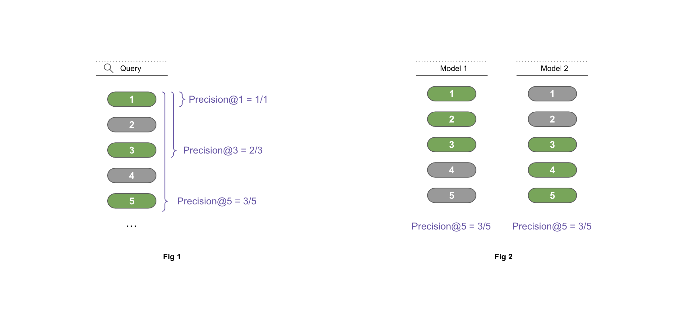
Precision fails to take into account the ordering of the relevant documents. For example consider the models A and B (Fig 2) where model A outputs [1,1,1,0,0](first 3 relevant) and model B outputs [0,0,1,1,1](indices 3-5 relevant); both the models get the same score Precision@5=3/5.

MAP@k: Mean Average Precision

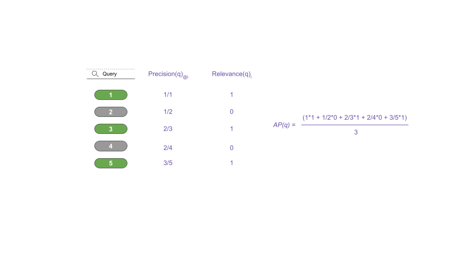
Average Precision(AP) evaluates whether all the relevant items selected by the model are ranked higher or not. Every time we find a relevant document, we look at the full picture of what came before.

MAP squeezes complex evaluation into a single number. It’s essentially the mean of AP over all the queries.

$$ AP@k(q) = \frac{\sum_{i=1}^k P(q)@i * rel(q)_i}{|rel(q)|} $$

$$ MAP@k(Q) = \frac{1}{|Q|} * \sum_{q\in Q} AP@k(q) $$

Where $\vert Q \vert$ is the number of queries, $P(q)@i$ is the precision of query q after first i documents, ${rel(q)_i}$ is the binary relevance of doc at position i, ${\vert rel(q) \vert}$ is the number of relevant documents.

MRR: Mean Reciprocal Rank

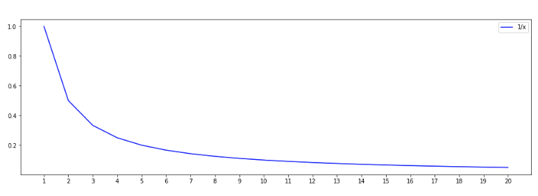
MRR puts focus on the first relevant document. It’s applicable when the system needs to return only the top matching document or the user only cares about the top result.

$$ MRR(Q) = \frac{1}{|Q|} * \sum_{q\in Q} \frac{1}{FirstRank(q)} $$

Where $\vert Q \vert$ is the number of queries and ${FirstRank(q)}$ is the returns the rank of first relevant dcuments for 1 query.

MRR(for 1 query) for different positions can be seen below. Notice the sharp fall in the values beyond the top few places.

1
2
3
4

import math

import matplotlib.pyplot as plt
%matplotlib inline

1
2
3
4
5

N = 20
plt.figure(figsize=(16, 5));
plt.plot(range(1, N+1), [1/n for n in range(1, N+1)], c="b", label="1/x");
plt.legend();
plt.xticks(range(1, N+1, 1));

** Note that the metrics related to Recall are not used in general because it is easy to achieve a recall of 100% by returning all documents for a query.

Graded labels

nDCG@k: Normalized Discounted Cumulative Gain

To understand nDCG, first let’s look at CG i.e. Cumulative Gain. We simply add up the relevance scores for top k documents returned for a query.

$$ CG@k(q) = \sum_{i=1}^k rel(q)_i $$

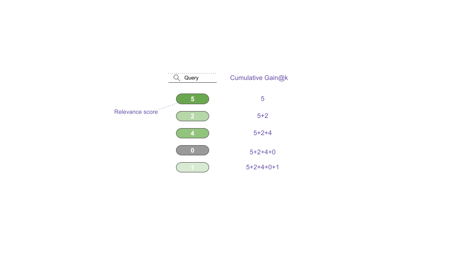
Note that CG does not take into account the position of the document. For example consider the models A and B where model A outputs [5,2,4,0,1] and model B outputs [2,0,5,1,4]; both the models get the same score CG@5=12.

DCG i.e. Discounted Cumulative Gain improves on CG by adding a discounting factor for each position.

$$ DCG@k(q) = \sum_{i=1}^k \frac{rel(q)_i}{log_2(i+1)} $$

here ${rel(q)_i}$ is the graded relevance of doc at position i.

 1
 2
 3
 4
 5
 6
 7
 8
 9
10
11
12
13
14
15
16
17
18
19
20
21
22
23
24
25
26
27
28
29

import math
from typing import List

import pandas as pd


def _get_dcg_at_k(scores: List[int]) -> pd.DataFrame:
    cols = ["position(i)", "relevance(i)", "log2(i+1)", "relevance(i) / log2(i+1)"]

    data = []
    for i, score in enumerate(scores):
        position = i + 1
        data.append((position, score, math.log2(position+1), score / math.log2(position+1)))

    return pd.DataFrame(data, columns=cols)


def get_dcg_at_k(scores: List[int]) -> None:
    df = _get_dcg_at_k(scores)
    
    dcg_so_far = ""
    for i, dcg in enumerate(df["relevance(i) / log2(i+1)"]):
        if not dcg_so_far:
            dcg_so_far = f"{dcg:2.2f}"
        else:
            dcg_so_far = f"{dcg_so_far} + {dcg:2.2f}"
        print(f"DCG@{i+1} = {dcg_so_far:<32} = {eval(dcg_so_far):2.2f}")
    
    return df

Now we can compare the results from the two models A and B we mentioned earlier.

1

get_dcg_at_k([5, 2, 4, 0, 1])  # model A

DCG@1 = 5.00                             = 5.00
DCG@2 = 5.00 + 1.26                      = 6.26
DCG@3 = 5.00 + 1.26 + 2.00               = 8.26
DCG@4 = 5.00 + 1.26 + 2.00 + 0.00        = 8.26
DCG@5 = 5.00 + 1.26 + 2.00 + 0.00 + 0.39 = 8.65

1

get_dcg_at_k([2, 0, 5, 1, 4])  # model B

DCG@1 = 2.00                             = 2.00
DCG@2 = 2.00 + 0.00                      = 2.00
DCG@3 = 2.00 + 0.00 + 2.50               = 4.50
DCG@4 = 2.00 + 0.00 + 2.50 + 0.43        = 4.93
DCG@5 = 2.00 + 0.00 + 2.50 + 0.43 + 1.55 = 6.48

DCG solves the problem with CG but it also has a drawback, it can’t be used to compare queries/models that return different number of results. For example consider query A and B where query A returns [5,2,4] query B returns [5,2,4,0,1];

1

get_dcg_at_k([5, 2, 4])  # query A

DCG@1 = 5.00                             = 5.00
DCG@2 = 5.00 + 1.26                      = 6.26
DCG@3 = 5.00 + 1.26 + 2.00               = 8.26

1

get_dcg_at_k([5, 2, 4, 0, 1])  # query B

DCG@1 = 5.00                             = 5.00
DCG@2 = 5.00 + 1.26                      = 6.26
DCG@3 = 5.00 + 1.26 + 2.00               = 8.26
DCG@4 = 5.00 + 1.26 + 2.00 + 0.00        = 8.26
DCG@5 = 5.00 + 1.26 + 2.00 + 0.00 + 0.39 = 8.65

Query B got higher DCG because it returned 5 documents whereas query A only returned 3. We can’t say that query B was better than query A. nDCG fixes this issue by adding a normalization factor on top of DCG.

$$ nDCG@k(Q) = \frac{1}{|Q|} * \sum_{q\in Q} \frac{DCG@k(q)}{DCG@k(sorted(rel(q)))} $$

Where $\vert Q \vert$ is the number of queries.

The normalization factor 𝐷𝐶𝐺@𝑘(𝑠𝑜𝑟𝑡𝑒𝑑(𝑟𝑒𝑙(𝑞))) is the Ideal DCG@k. This is calculated by sorting the graded relevance scores returned for a query and then calculating the DCG@k. nDCG@k always lie between 0 and 1.

Now we can compare queries/models with different number of results.

1

get_dcg_at_k(sorted([5, 2, 4], reverse=True))  # Ideal DCG@k for query A

DCG@1 = 5.00                             = 5.00
DCG@2 = 5.00 + 2.52                      = 7.52
DCG@3 = 5.00 + 2.52 + 1.00               = 8.52

nDCG@3 for query A = 8.26 / 8.52 = 0.9694

1

get_dcg_at_k(sorted([5, 2, 4, 0, 1], reverse=True))  # Ideal DCG@k for query B

DCG@1 = 5.00                             = 5.00
DCG@2 = 5.00 + 2.52                      = 7.52
DCG@3 = 5.00 + 2.52 + 1.00               = 8.52
DCG@4 = 5.00 + 2.52 + 1.00 + 0.43        = 8.95
DCG@5 = 5.00 + 2.52 + 1.00 + 0.43 + 0.00 = 8.95

nDCG@5 for query B = 8.65 / 8.95 = 0.9664

References

[1] Sebastian Hofstätter. “Advanced Information Retrieval 2021 @ TU Wien”

[2] Amit Chaudhary. https://amitness.com/2020/08/information-retrieval-evaluation